Level Up Your Code: Essential Software Quality Metrics
This listicle presents seven essential software quality metrics your team should track to improve your development process and product quality. Understanding metrics like Cyclomatic Complexity, Code Coverage, Defect Density, Mean Time to Failure (MTTF), Technical Debt Ratio, Maintainability Index, and Lead Time for Changes is critical for delivering high-quality software. These software quality metrics offer actionable insights into your codebase's health and maintainability, ultimately leading to better products and more efficient teams.
1. Cyclomatic Complexity
Cyclomatic Complexity, a crucial software quality metric, provides valuable insights into the structural intricacy of your code. By analyzing the number of linearly independent paths through a program's control flow, it quantifies complexity based on decision points like if-else statements, loops, and switch cases. A higher Cyclomatic Complexity score indicates more paths through the code, suggesting increased difficulty in testing, maintaining, and understanding that particular piece of code. This metric empowers development teams to proactively identify potential problem areas and prioritize refactoring efforts for improved code quality and maintainability.
Cyclomatic Complexity operates by examining the control flow graph of a program. Each node in this graph represents a block of sequential code, and edges represent the transfer of control between these blocks. The more branches and loops present, the more complex the graph becomes, resulting in a higher Cyclomatic Complexity score. This metric is language-agnostic, making it applicable to any programming language and promoting consistent code quality analysis across diverse projects. The numerical value generated by the Cyclomatic Complexity analysis directly indicates the minimum number of test cases required for complete path coverage, providing a practical estimate of testing effort.
For Engineering Managers, Scrum Masters, and Agile Coaches, Cyclomatic Complexity offers a quantifiable measure for evaluating code quality and technical debt, assisting in sprint planning and risk assessment. Product Owners and CTOs can leverage this metric to understand the maintainability of the codebase and the potential impact on project timelines and budgets. Software Development Teams, Jira Users, and DevOps Leaders benefit from integrating Cyclomatic Complexity analysis into their CI/CD pipelines, allowing for automated monitoring and early detection of overly complex code. Team Leads in Agile Environments can use this metric during code reviews to facilitate focused discussions on code structure and maintainability, driving improvements in overall code quality. Atlassian Marketplace Buyers can find various plugins that integrate Cyclomatic Complexity analysis into their existing workflows.
Several organizations have successfully implemented Cyclomatic Complexity analysis in their development processes. Microsoft, for example, incorporates Cyclomatic Complexity thresholds into their development guidelines, ensuring code maintainability across their vast codebase. SonarQube, a popular static code analysis platform, provides seamless integration of Cyclomatic Complexity analysis into enterprise CI/CD pipelines. Even NASA leverages Cyclomatic Complexity limits in their software development standards for mission-critical code, highlighting the importance of this metric in high-stakes environments.
Pros of using Cyclomatic Complexity:
- Predictive Power: Strong indicator of testing effort and future maintenance difficulties.
- Targeted Refactoring: Helps pinpoint areas of code that require refactoring.
- Wide Tool Support: Readily available in many development tools and IDEs.
- Easy Interpretation: Provides an objective, easy-to-understand numerical score.
- Defect Correlation: Correlates well with the likelihood of defects in the code.
Cons of using Cyclomatic Complexity:
- Limited Scope: Doesn't consider data complexity or algorithmic efficiency.
- Potential for Misuse: May encourage artificial code splitting without addressing underlying design issues.
- Gamification Risk: Developers might focus solely on reducing the number without considering overall design improvements.
- Structural Focus: Measures only structural complexity, not the overall code quality.
Tips for effective utilization of Cyclomatic Complexity:
- Establish Thresholds: Define acceptable complexity limits (typically 10-15 for most codebases).
- Prioritize Refactoring: Concentrate on reducing complexity in frequently modified code sections first.
- Code Review Integration: Utilize complexity metrics during code reviews to guide discussions and promote best practices.
- Combine with other Metrics: Integrate with other metrics like test coverage for a more comprehensive understanding of code quality.
By understanding and utilizing Cyclomatic Complexity effectively, development teams can improve code maintainability, reduce testing effort, and enhance the overall quality of their software. It's a valuable tool in any software development arsenal and deserves its place amongst the top software quality metrics.
2. Code Coverage
Code coverage is a crucial software quality metric that measures the percentage of your source code executed during automated testing. It provides a quantitative assessment of how thoroughly your test suite exercises the codebase, shining a light on both well-trodden and unexplored code paths. By identifying gaps in testing, code coverage helps teams pinpoint potential vulnerabilities and improve the overall reliability of their software. This makes it an invaluable tool for Engineering Managers, Scrum Masters, Agile Coaches, Product Owners, CTOs, Software Development Teams, and DevOps Leaders striving to deliver high-quality products.
Code coverage analysis works by instrumenting the code and tracking which lines, branches, functions, or statements are executed when tests run. This instrumentation can be done at compile time, load time, or even runtime, depending on the tools and programming language used. The results are typically presented as a percentage, with higher percentages indicating more comprehensive testing. Different coverage types provide varying levels of granularity:
- Line Coverage: The percentage of lines of code executed. This is the most basic and commonly used metric.
- Branch Coverage: The percentage of code branches (e.g., if-else conditions) executed. This helps ensure that all possible execution paths within a given block of code are tested.
- Function Coverage: The percentage of functions or methods called during testing. This verifies that all defined functions are used at least once.
- Statement Coverage: Similar to line coverage, but focuses on the execution of individual statements within a line of code. This is particularly relevant in languages where a single line can contain multiple statements.
Several tools automate code coverage analysis and integrate seamlessly into CI/CD pipelines, providing real-time feedback during test execution. These tools often offer visual highlighting of covered and uncovered code within the IDE and allow for trend tracking over time to monitor testing improvements. This automated reporting and visual feedback are incredibly valuable for Jira users and Team Leads in Agile Environments, allowing them to quickly identify and address testing gaps.
Companies like Spotify, Netflix, and Google leverage code coverage metrics to enhance their software quality. Spotify, for example, maintains over 80% code coverage across its microservices architecture. Netflix uses coverage data to inform their testing strategy for their streaming platform. Google even enforces coverage requirements for critical infrastructure components, underscoring the importance of this metric for maintaining robust and reliable systems.
While code coverage offers numerous advantages, it is crucial to understand its limitations. High coverage doesn't automatically guarantee high-quality tests. It's possible to achieve high coverage with superficial tests that don't effectively uncover bugs. Focusing solely on increasing coverage can lead to a "checkbox mentality," where developers write tests simply to meet a target percentage rather than to thoroughly test the code's logic. Furthermore, code coverage doesn't measure test effectiveness or bug detection capability. It can even create a false sense of security if poor-quality tests give the illusion of comprehensive coverage.
To effectively utilize code coverage, aim for a practical target of 70-80% for most projects. Prioritize covering critical business logic and error handling paths. Use coverage reports to guide test writing and identify gaps, but don't rely on it as the sole quality measure. Combining code coverage with other techniques like mutation testing, which assesses the effectiveness of tests in detecting changes in the code, provides a more robust evaluation of software quality.
For Java development, JaCoCo is a widely used library. JavaScript developers often rely on Istanbul/NYC. Coverage reporting platforms like Codecov and Coveralls further streamline the process by providing centralized dashboards and integration with various CI/CD systems. By carefully incorporating code coverage into your development workflow and understanding its strengths and limitations, you can leverage this metric to improve the quality and reliability of your software. This ultimately benefits Atlassian Marketplace Buyers and all stakeholders by ensuring the delivery of robust and dependable products.
3. Defect Density
Defect density is a crucial software quality metric that provides insights into the concentration of defects within a given piece of code. It's calculated by dividing the number of confirmed defects by the size of the software, typically measured in thousands of lines of code (KLOC) or function points. This normalization by code size allows for meaningful comparisons of quality across different modules, projects, and even releases, making it a cornerstone of many quality improvement initiatives and benchmarking exercises. For engineering managers, scrum masters, and development teams striving for continuous improvement, defect density offers a quantifiable way to assess and track code quality.
This metric works by providing a standardized way to express the prevalence of bugs. Instead of simply stating a raw number of defects, which can be misleading when comparing projects of varying sizes, defect density puts everything on a level playing field. A smaller module with 10 defects in 1 KLOC has a much higher defect density (10 defects/KLOC) than a larger module with 50 defects in 10 KLOC (5 defects/KLOC), even though the latter has a larger absolute number of defects. This normalized perspective highlights areas of concern more effectively.
Several key features contribute to the power of defect density as a quality metric. Firstly, it facilitates trend analysis. By tracking defect density across multiple releases, teams can monitor the effectiveness of quality improvement efforts and identify potential regressions. Secondly, it enables benchmarking, both internally against past performance and externally against industry standards. This allows teams to assess their standing within the broader development landscape and identify areas for improvement. Finally, defect density helps pinpoint high-risk modules. A module with a significantly higher defect density than others is likely to require more thorough testing, review, or even refactoring.
Defect density offers several compelling advantages. Its objectivity allows for unbiased assessments of code quality, promoting data-driven decision-making. It enables meaningful comparisons between projects of different scales, facilitating resource allocation and prioritization. Furthermore, by identifying areas prone to defects, defect density helps focus testing and review efforts, leading to more efficient use of resources. Over time, consistent tracking of defect density provides valuable data for predicting maintenance costs and effort, allowing for better project planning and budgeting.
However, like any metric, defect density has its limitations. Its accuracy is highly dependent on the effectiveness of defect detection and the consistency of defect reporting. Variations in defect classification standards across teams or organizations can skew comparisons. Moreover, defect density doesn't inherently consider the severity or business impact of the defects. A module with a high density of minor, cosmetic bugs might appear worse than a module with a lower density of critical, show-stopping bugs. Finally, there’s the risk of manipulation. Teams might be tempted to underreport defects or artificially inflate code size to improve their perceived defect density.
Successful implementations of defect density can be found in various industries. IBM reports industry averages ranging from 1 to 25 defects per KLOC, demonstrating the metric's widespread use and the influence of development methodology on defect rates. Microsoft utilizes defect density to guide resource allocation across different components of Windows, ensuring that areas with higher defect concentrations receive appropriate attention. In the automotive industry, where software failures can have life-threatening consequences, the ISO 26262 standard mandates specific defect density targets for safety-critical systems, highlighting the metric's importance in ensuring high reliability.
To leverage the full potential of defect density, teams should adhere to a few best practices. Establishing consistent defect classification and counting standards across the organization is paramount. Tracking defect densities for both pre-release and post-release phases offers a comprehensive view of software quality. Using defect density to identify modules requiring more rigorous code reviews or refactoring is a proactive approach to quality improvement. Finally, consider incorporating defect severity weighting into the metric to gain a more nuanced understanding of the true impact of defects. This could involve assigning weights to different defect categories and calculating a weighted defect density that reflects both the quantity and the severity of the issues. By following these tips, teams can effectively utilize defect density to drive continuous improvement in software quality and deliver more robust and reliable products.
4. Mean Time to Failure (MTTF)
Mean Time to Failure (MTTF) is a crucial software quality metric that measures the average time a system runs before experiencing a critical failure. It provides a quantifiable measure of system reliability and stability, allowing teams to predict potential downtime, schedule maintenance, and ultimately, improve the user experience. For engineering managers, scrum masters, product owners, and software development teams working in agile environments, understanding and utilizing MTTF is essential for delivering high-quality, dependable software. It's a key indicator of how well a system performs over time, helping organizations meet service-level agreements (SLAs) and build customer trust. This makes it a deserving addition to any list of essential software quality metrics.
MTTF focuses on systems that cannot be repaired or are not intended for repair, such as hardware components or specific software releases. The calculation involves observing multiple identical systems over a period of time, recording the time to failure for each, and then calculating the average. In a software context, this could mean tracking multiple deployments of the same version and measuring the time until a critical error occurs. The higher the MTTF, the more reliable the system is considered to be.
How MTTF Works in Practice:
MTTF provides a valuable perspective on software reliability by tracking the time between failures. Let’s say you deploy a new version of your software. By tracking the time until a critical failure occurs across multiple instances of this deployment, you can calculate the MTTF. This helps you understand the overall reliability of that specific release. Tracking MTTF trends over time, particularly after implementing bug fixes or performance enhancements, helps quantify the impact of these changes on system stability. This data-driven approach to reliability empowers teams to make informed decisions regarding future development and maintenance.
Successful Implementation Examples:
Several organizations effectively utilize MTTF to ensure high availability and reliability. AWS, for instance, leverages MTTF to track the performance of their cloud services and maintain their stringent 99.99% uptime SLAs. Similarly, Netflix, with its complex microservices architecture, relies on MTTF measurements across different services to ensure the reliability of their streaming platform. In the financial sector, banking systems employ MTTF to guarantee the dependable processing of transactions, a critical requirement in this industry. These examples highlight the applicability of MTTF across diverse industries and system complexities.
Actionable Tips for Utilizing MTTF:
To effectively utilize MTTF, consider these practical tips:
- Define 'Failure' Clearly: Establish precise criteria for what constitutes a "failure" within your system. This ensures consistent measurement and meaningful analysis. Is it a complete system outage, a specific error code, or a degradation in performance beyond a defined threshold? A clear definition is paramount.
- Track Trends: Focus on MTTF trends over time rather than isolated measurements. This provides a more comprehensive understanding of system reliability and the impact of changes.
- Segment by Severity and Component: Segment MTTF data by failure severity (critical, major, minor) and system components. This allows for targeted improvements and better resource allocation.
- Prioritize Improvements: Use MTTF data to prioritize reliability improvement efforts. Focus on components or areas with the lowest MTTF and highest impact on users.
When and Why to Use MTTF:
MTTF is particularly valuable in the following scenarios:
- Predictive Maintenance: MTTF helps predict when failures are likely to occur, enabling proactive maintenance scheduling and minimizing downtime.
- SLA Management: Use MTTF data to define and monitor compliance with service-level agreements.
- Reliability Benchmarking: Compare the reliability of different systems or components using MTTF as a benchmark.
- Capacity Planning: MTTF data supports informed capacity planning by providing insights into system stability and potential failure rates.
Pros and Cons of MTTF:
Pros:
- Provides a clear and quantifiable measure of system reliability for stakeholders.
- Facilitates proactive maintenance planning and resource allocation.
- Supports SLA definition and compliance monitoring.
- Enables comparison of reliability across different systems.
Cons:
- Requires extended observation periods for accurate measurements.
- May not effectively capture infrequent or intermittent failures.
- Can be influenced by external factors such as usage patterns and environment.
- Doesn't inherently distinguish between different failure types.
Despite its limitations, MTTF remains a valuable metric for understanding and improving software reliability. By implementing the tips provided and understanding the context of its application, teams can leverage MTTF to build more robust and dependable software systems. This translates to enhanced user satisfaction, reduced operational costs, and a stronger competitive advantage.
5. Technical Debt Ratio
Technical Debt Ratio is a crucial software quality metric that quantifies the amount of technical debt present in a codebase. It expresses this debt as a percentage of the total estimated effort required to develop the application from scratch. Essentially, it measures the cost to fix all existing maintainability issues relative to the cost of rewriting the entire software. This metric helps teams understand the long-term implications of taking shortcuts during development and enables them to prioritize refactoring efforts effectively. By providing a quantifiable measure of technical debt, it bridges the gap between technical concerns and business decisions, facilitating informed discussions and resource allocation.

The Technical Debt Ratio aggregates multiple code quality issues, including code smells, bugs, and design flaws, into a single, easily digestible metric. This consolidated view simplifies complex technical details, making it easier for non-technical stakeholders to grasp the overall health of the software. The ratio can be tracked over time, providing insights into the accumulation or reduction of technical debt across different releases or sprints. This trend analysis allows teams to monitor the impact of their development practices and assess the effectiveness of their refactoring efforts. By translating technical concepts into a business-friendly percentage, the Technical Debt Ratio facilitates communication and collaboration between development teams and business stakeholders, enabling more informed decision-making regarding technical investments.
Several well-known organizations leverage the Technical Debt Ratio for managing their software quality. SonarQube, a popular static analysis platform, calculates this metric for thousands of enterprise projects, providing valuable insights into code health and maintainability. PayPal has utilized technical debt metrics, including the Technical Debt Ratio, to guide their platform modernization efforts, ensuring sustainable development practices. Similarly, Atlassian tracks the debt ratio across their product portfolio to inform maintenance planning and resource allocation. These examples showcase the practical application and benefits of incorporating this metric into the software development lifecycle.
When considering implementing the Technical Debt Ratio, understanding its strengths and weaknesses is essential. One of its key advantages is the ability to translate complex technical issues into easily understandable business terms. This facilitates communication with stakeholders and helps justify investments in refactoring and code improvement initiatives. The metric also provides a clear target for technical debt reduction, enabling teams to set goals and track progress effectively. However, accurately estimating the cost of remediating all technical debt can be challenging, leading to potential inaccuracies in the calculated ratio. Moreover, simplifying complex technical quality issues into a single percentage may sometimes oversimplify the underlying problems. It's important to remember that the ratio doesn't account for the business value of features that might contribute to the technical debt. Different static analysis tools might also employ varying calculation methods, making direct comparisons challenging.
To effectively leverage the Technical Debt Ratio, consider these practical tips. Establish clear targets for your technical debt ratio. A ratio of less than 5% is often considered a benchmark for healthy codebases. Prioritize addressing technical debt in frequently changed areas of the codebase, as these areas are more prone to accumulating further debt and experiencing increased maintenance costs. Use the trends in your debt ratio to inform sprint planning decisions, allocating resources for refactoring and code improvement as needed. Combine the Technical Debt Ratio with other code quality metrics, such as cyclomatic complexity, to gain deeper insights into the specific areas requiring attention. By incorporating these strategies, teams can effectively manage technical debt and improve the overall quality and maintainability of their software.
The concept of technical debt, analogous to financial debt, was introduced by Ward Cunningham. Martin Fowler further popularized the concept and advocated for its importance in software development. SonarSource, through their technical debt model and tools like SonarQube, played a significant role in defining and popularizing the Technical Debt Ratio as a key software quality metric. This metric is especially relevant for Engineering Managers, Scrum Masters, Agile Coaches, Product Owners, CTOs, Software Development Teams, Jira Users, DevOps Leaders, and Team Leads in Agile Environments looking to maintain high software quality and manage technical debt effectively. By using the Technical Debt Ratio, teams can make data-driven decisions, prioritize improvements, and ensure the long-term health and sustainability of their software projects.
6. Maintainability Index
Maintainability Index (MI) is a crucial software quality metric that provides a consolidated view of how easy it is to maintain and modify a particular codebase. Unlike individual metrics that focus on specific aspects of code quality, MI combines several factors into a single score, making it easier to grasp the overall maintainability picture and communicate it to both technical and non-technical stakeholders. This metric helps teams prioritize refactoring efforts, track improvements over time, and ensure code remains manageable as software evolves.
MI typically incorporates metrics such as cyclomatic complexity (which measures the number of independent paths through a piece of code), lines of code, Halstead volume (a measure of program size and complexity based on the number of operators and operands), and sometimes comment percentage. These individual metrics are combined using a formula to produce an MI score, typically ranging from 0 to 100. Higher scores indicate better maintainability. A high MI suggests the code is well-structured, understandable, and easy to modify, while a low MI signals potential maintenance challenges. This allows teams to pinpoint areas requiring attention and proactively address potential issues before they become costly problems.
For example, Microsoft Visual Studio integrates MI directly into its code analysis tools, allowing developers to see the MI score for their code in real-time. Enterprise teams utilize MI to prioritize code review efforts, focusing on modules with low MI scores that pose the greatest maintenance risk. During legacy system modernization projects, MI is tracked over time to demonstrate the impact of refactoring and modernization activities on the overall maintainability of the system. This allows stakeholders to quantify the improvements made and justify continued investment in modernization.
Several factors contribute to MI's prominent place amongst software quality metrics. Its ability to simplify complex quality assessments into a single, easily interpretable number makes it particularly valuable for communicating with non-technical stakeholders. Furthermore, MI provides a consistent measurement across different codebases, facilitating comparisons and benchmarking efforts. The metric is also widely supported by various static analysis tools, making it readily accessible to development teams.
However, MI also has some limitations. By combining multiple metrics into a single score, it can obscure important details about specific areas of concern. Different calculation methods for MI can yield different results, making it essential to understand which method is being used. The weights assigned to component metrics in the MI calculation may not be suitable for all contexts, potentially undervaluing certain aspects of maintainability. Finally, developers could potentially "game" the system by optimizing for individual component metrics without actually improving the overall maintainability of the code.
Here are some practical tips for using the Maintainability Index effectively:
- Focus on Trends: Track MI trends over time to identify improving or declining maintainability rather than relying on absolute values.
- Investigate Underlying Metrics: When MI scores are concerning, delve into the underlying metrics (cyclomatic complexity, lines of code, etc.) to pinpoint the root causes.
- Set Thresholds: Establish MI thresholds for code review triggers. A common practice is to flag code with an MI below 10 as high risk, requiring mandatory review.
- Granular Analysis: Track MI at both the file and method levels for more granular insights into maintainability issues.
The following infographic visually represents the typical interpretation of Maintainability Index scores, categorized into three ranges.
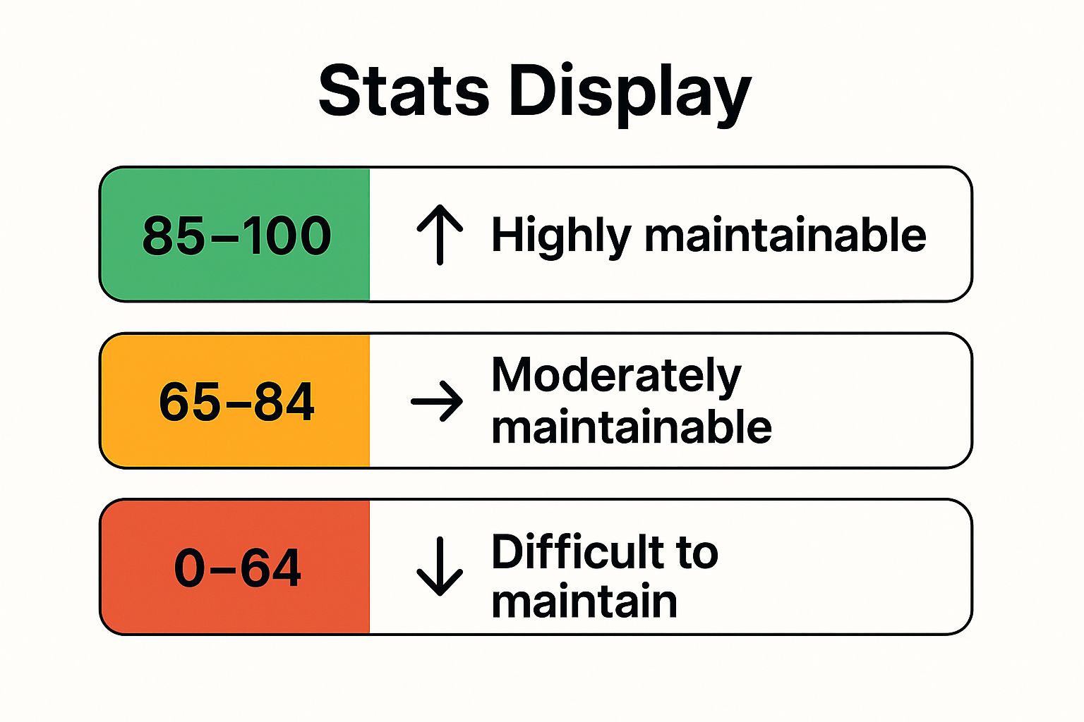
The infographic clearly illustrates the relationship between MI scores and maintainability, highlighting the ranges indicating high, moderate, and low maintainability. Scores between 85 and 100 represent highly maintainable code, while scores below 65 signify code that is difficult to maintain and likely to require significant refactoring. This visual representation makes it easy to understand the significance of MI scores and prioritize code maintenance efforts. The MI, popularized by Microsoft through its integration into Visual Studio, the Software Engineering Institute (SEI), and the original research by Oman and Hagemeister, offers a valuable tool for assessing and improving the long-term health and sustainability of software projects. By understanding and leveraging this metric, teams can build more robust, maintainable, and cost-effective software solutions.
7. Lead Time for Changes
Lead Time for Changes is a crucial software quality metric that measures the time elapsed between committing a code change and its successful deployment to production. This metric provides a powerful insight into the efficiency of your entire software delivery pipeline, reflecting how quickly your team can deliver value to users. It encompasses all stages of the process, from development and testing to deployment and release, offering a holistic view of your delivery performance. This makes it a key metric for anyone involved in software development, from engineering managers and scrum masters to CTOs and product owners. As a software quality metric, it focuses not just on the quality of the code itself, but also on the quality and efficiency of the processes surrounding its delivery. This positions Lead Time for Changes as a vital indicator of organizational agility and responsiveness to market demands, justifying its inclusion in this list of essential software quality metrics.
Understanding Lead Time for Changes is essential for organizations striving to optimize their software delivery performance. It offers a quantifiable measure of how quickly your team can respond to user needs, market changes, and business requirements. A shorter lead time translates to faster feedback loops, quicker iterations, and ultimately, a more competitive edge in the market. This is particularly important in today’s fast-paced digital landscape, where the ability to deliver value rapidly is often a key differentiator.
How It Works:
Lead Time for Changes is tracked from the moment a developer commits a code change to the version control system (e.g., Git) until the moment that change is successfully running in the production environment. This includes the time spent in code review, testing (unit, integration, system, user acceptance testing), staging, and final deployment. It’s important to measure the entire process to get a true picture of your delivery pipeline efficiency.
Features and Benefits:
- End-to-End Measurement: Provides a comprehensive view of the entire delivery process, from code commit to production deployment.
- Bottleneck Identification: Helps pinpoint bottlenecks and inefficiencies within the development pipeline. By analyzing the time spent in each stage, teams can identify areas for improvement and optimization.
- Performance Indicator: Serves as a key indicator of organizational software delivery performance and overall agility.
- Benchmarking: Allows organizations to benchmark their performance against industry standards and identify areas for improvement.
- Granular Measurement: Can be measured at different levels of granularity, such as individual commits, features, or releases, providing a more nuanced understanding of delivery performance.
Pros and Cons:
Pros:
- Clear measure of delivery speed and efficiency.
- Helps identify bottlenecks in the development pipeline.
- Correlates with organizational performance and competitiveness.
- Motivates process improvement and automation.
- Enables benchmarking against industry standards.
Cons:
- May encourage rushing changes without proper quality checks if not balanced with other quality metrics.
- Can be influenced by variations in change size and complexity.
- Requires well-implemented tracking systems and process discipline.
- Might not account for delays caused by business prioritization.
Examples of Successful Implementation:
- Elite Performers (DORA): Organizations identified as "elite performers" by DORA achieve lead times of less than one hour, demonstrating exceptional agility and efficiency in their delivery pipelines.
- Netflix: Netflix is renowned for its ability to deploy thousands of changes daily with minimal lead time, enabling them to constantly innovate and improve their streaming service.
- Amazon: Amazon's impressive deployment frequency, averaging one deployment every 11.7 seconds across their services, highlights the power of automation and optimized delivery pipelines.
Actionable Tips for Improvement:
- Automate: Automate as much of the development and deployment pipeline as possible, from testing to deployment.
- Segment Measurement: Measure lead time for different types of changes (e.g., bug fixes, features) separately to identify specific areas for improvement.
- Reduce Batch Sizes: Focus on reducing the size of changes and increasing deployment frequency to minimize risk and improve feedback loops.
- Monitor Trends: Track lead time trends over time and investigate any significant increases to proactively address potential issues.
- Implement Continuous Integration/Continuous Delivery (CI/CD): Adopt CI/CD practices to streamline the development and deployment process.
When and Why to Use This Approach:
Lead Time for Changes should be a key metric for any organization developing and deploying software. It provides a critical measure of agility and efficiency, helping teams identify bottlenecks and optimize their delivery pipelines. This metric is particularly important for organizations adopting Agile and DevOps methodologies, where rapid and frequent deployments are essential.
Lead Time for Changes is popularized by DORA (DevOps Research and Assessment) and features prominently in the Google Cloud State of DevOps Report. It's also a key concept discussed in the influential book "Accelerate" by Nicole Forsgren, Jez Humble, and Gene Kim. Tracking and improving this metric is a vital step towards building a high-performing software delivery organization.
Software Quality Metrics Comparison
| Metric |
⭐ Expected Outcomes |
🔄 Implementation Complexity |
⚡ Resource Requirements |
💡 Ideal Use Cases |
📊 Key Advantages |
| Cyclomatic Complexity |
Measures control flow complexity; predicts testing effort and maintainability |
Medium; requires static code analysis tools |
Low to medium; tooling widely available |
Identifying complex code needing refactoring |
Objective, language-independent, well-supported |
| Code Coverage |
Measures test completeness; identifies untested code areas |
Medium; requires instrumentation and test integration |
Medium; needs test suites and CI/CD integration |
Ensuring thorough test suites and regulatory compliance |
Objective measure of test coverage; visual feedback |
| Defect Density |
Tracks defects per size unit; assesses code quality trends |
Low; depends on accurate defect tracking |
Low; requires defect and code size data collection |
Benchmarking code quality and prioritizing reviews |
Normalizes defects by size; predicts maintenance effort |
| Mean Time to Failure (MTTF) |
Measures system reliability and stability over time |
Medium; needs failure logging and monitoring setup |
Medium; requires monitoring and failure data |
Measuring operational reliability and planning maintenance |
Clear reliability metric; supports SLA and maintenance |
| Technical Debt Ratio |
Quantifies debt as % of dev effort; impacts maintainability |
Medium; requires static analysis and cost estimation |
Medium; integrates with code quality tools |
Prioritizing refactoring and justifying investments |
Translates technical issues to business terms |
| Maintainability Index |
Composite maintainability score (0-100 scale) |
Medium; combines multiple metrics |
Medium; needs integration of metrics |
Tracking code maintainability trends and prioritizing refactor |
Simplifies quality assessment; easy communication |
| Lead Time for Changes |
Measures time from commit to production; reflects delivery speed |
Medium to high; needs pipeline instrumentation |
Medium to high; requires CI/CD and tracking tools |
Assessing development and deployment efficiency |
Clear delivery speed metric; identifies bottlenecks |
Putting Metrics to Work: Improving Your Software Quality Journey
This article explored seven key software quality metrics—Cyclomatic Complexity, Code Coverage, Defect Density, Mean Time to Failure (MTTF), Technical Debt Ratio, Maintainability Index, and Lead Time for Changes—providing a foundation for understanding and improving your software development lifecycle. These metrics offer invaluable insights into various aspects of your codebase, from identifying potential bugs and maintainability issues to assessing overall reliability and performance. The most important takeaway is that utilizing these software quality metrics empowers you to make data-driven decisions, optimize your development processes, and ultimately deliver higher-quality software.
Mastering these concepts and integrating them into your workflow translates to tangible benefits: reduced development costs, faster time to market, and increased customer satisfaction. By proactively addressing code quality bottlenecks identified through these metrics, you can prevent costly rework down the line, streamline your development pipeline, and build more robust and maintainable software. Remember, effective implementation involves setting realistic targets, fostering collaborative review processes, and continuous monitoring. Tailoring your approach to your specific context is crucial for success.
Effective software quality management isn't a destination, but a continuous journey of improvement. Embracing data-driven insights provided by software quality metrics empowers your team to build better software, faster, and more efficiently. Want to streamline your metrics tracking and gain actionable insights into your software quality? Explore Umano, a platform designed to help you measure, analyze, and improve your development process. Visit Umano to learn more and start optimizing your software quality journey today.